ESO NTT+SOFI Data Processing
for Linearity and Shade

Background
SOFI is an infrared imager and low resolution spectrograph on the ESO NTT. It provides imaging with ~0.248" pixels on a 1024x1024 HgCdTe detector. The official ESO SOFI pages (at the time of writing) can be found at http://www.ls.eso.org/lasilla/sciops/ntt/sofi/index.html
My initial concern when I started an astrometric program with SOFI was measuring its non-linearity, and applying a correction for it.
There were two problems in doing this
1.The available data to measure the non-linearity wasn't so crash hot, and
2.the 'zero-point' level of SOFI is only a loosely defined concept.
As a result the best advice I got was "don't exceed 10,000adu per pixel, and then its pretty much linear". Naturally, I wanted to check this out for myself, so I took some measurements. Before describing them, however, I need to go a bit further into the second point above - what is the zero-point of a SOFI exposure?
This page presents somewhat more detail than I was able to fit into my published paper discussing these effects - Tinney et al. 2003, AJ, 126, 975.
SOFI zero-points and the "shade" pattern
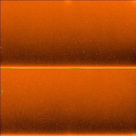
It turns out that the zero-point image (ie the image you'd get from an exposure on which zero-flux is incident - usually roughly approximated by a dark frame), is very non-flat. The non flatness is primarily in the vertical direction (a pattern called the shade), with other much lower 'intensity' patterns in both X and Y due to read-out register glow in the top, right corner of each qudrant of the detector (several tens of adu in spots of 10-50 pixels in diameter), and a 'ray' pattern dark image covering the entire detector with an intensity of a few adu.
A SOFI dark. Notice the vertical 'shading' pattern, as well as the bright register readout spots in the top-right corners of the quadrants.
If you extract the vertical profile (by medianning to remove the bad pixels, cosmic rays etc) and subtract that from the dark, you can more clearly see the read-out register glow (which is a function of exposure parameters) and the 'ray' pattern (which seems to be pretty constant regardless of readout parameters. So I just make one ray pattern for an entire run and subtract it from all images.

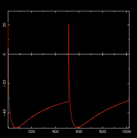
And the actual vertical shade pattern looks like this
The major problem is that both the overall level of the shade, and its non-flatness, are strong functions of the overall flux incident on the detector. The following image highlights this. It shows the shade pattern for a series of images as a function of the mean flux per pixel (averaged over the entire image). (I explain how I derived these below).
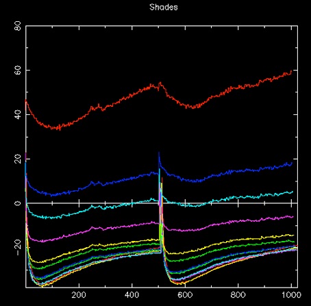
An example of how the shade changes as a function detector illumination. In these examples the mean illumination levels in adu/pix averaged over the entire 1024x1024 image (from the top down) are:
3199(red),
2221(blue),
1861(cyan),
1467(magenta),
1086(yellow),
958(green)
701(blue),
685(green),
554(cyan),
483(magenta),
226(yellow) and
87(red).
This means that for an arbitrary exposure, you have no way of knowing what number of adu in a given pixel corresponds to zero flux! This means you can never get your flat-fielding exactly right ot very high precision, and if there's non-linearity present, you don't know precisely how many photons you've counted in order to apply a non-linearity correction.
This is usually not seen as a killer problem in most applications, as observers simply acquire groups of images closely spaced in time with similar levels of illumination - the 'shade' patterns for all these images will be very similar. By creating a 'sky' from this image, and subtracting it from all the images in the group, you'll also be subtracting close to the correct shade pattern (as long as the sky is not varying too much). For most observers linearity corrections at the 1-2% level are not seen as critical in the infrared, so they just don't care at that sort of level. However, it could be critical to my program.
Removing the Dark 'Ray' pattern
I create a single 'ray' image from dark frames with similar readout parameters (DIT & NDIT) to my observations by subtracting a medianned 'shade' profile (like the first plot shown above) to produce an image like that shown above. This is subtracted from all data frames.
Removing Inter-quadrant Cross-talk
This effect is quite serious in SOFI (if you don't know what it is see the SOFI Manual) but can be removed with a very simple data processing procedure. There is a MIDAS script to do this, but I created my own script (esoxtalk) for processing in Figaro. I find a cross-talk coefficient of 2.5e-5 works well.
Calibrating the shade
Then the next step is to remove a shade pattern from every image.
What I have been doing is obtaining calibration shades at a large range of illumination levels, and then picking the closest illumination level to each group of frames I process, and subtract that from each of them. The actual illumination level in each image will not be precisely the same as the illumination level used to derive the shade correction, but it should be better than doing nothing.
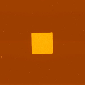
Shade calibrations are obtained as part of the 'Special Dome Flat' OB on the NTT. Observations of both an illuminated and unilluminated dome flat screen are obtained with the focal plane mask correctly positioned, and with the focal plane mask slightly out of position. The latter means that most of the CCD is illuminated as a flat-field, but a vertical strip of a few hundred pixels is left dark. The shade pattern can be extracted from this dark strip. The image below shows an example of this type of image.
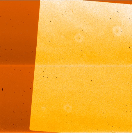
Vertical median-combined cuts through images like this, with the lamp brightness suitably adjusted were used to create the "swathe" of shade patterns shown above.
An interesting question to ask is whether there is a simple functional form to the two dimensional surface defined by the "swathe" of shade patterns - if there is you can create a calibration which can remove the shade from ANY image with greatly reduced systematic effects.
To examine this I looked at the value of the shade pattern for selected Y-values in the swathe, as a function of illumination levels. (Note that when I say illumination level I mean the total number of ADU collected in the entire array (ie summing over all 1024x1024 pixels), which I normalise by the number of pixels (1024x1024). This is not the same as the mean illumination level in the illuminated portion of the image above.)
I chose a bunch of Y values, and derived the mean value of each shade in the range Y-5 to Y+5. The resulting family of curves is shown below (and is available in Postscript). The fitted curves to each set of data points are cubic polynomials.
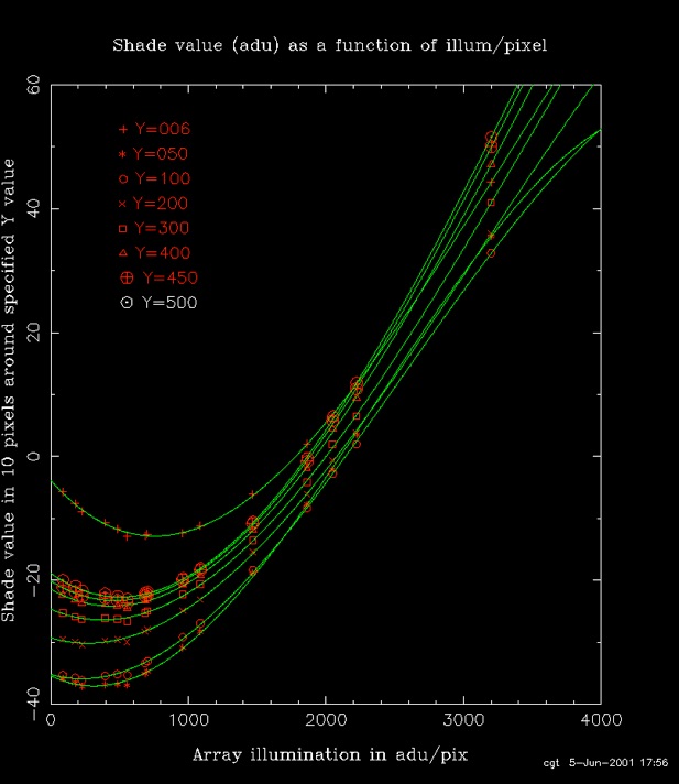
What we see is that for each Y value we can produce a cubic polynomial interpolation! So it is possible to produce a set of 1024 cubic polynomials which can subtract the shade pattern to better than an ADU everywhere on the detector. This is the technique described in Tinney et al. 2003, AJ, 126, 975.
Linearity Correction
All detectors are non-linear at some level (yes even CCDs). HgCdTe devices are particularly renowned for their non-linearity, which increases markedly at high count levels. There are no current results available for non-linearity in SOFI in the available documentation. However the recommendation is that if you keep counts below ~10,000adu per pixel, non-linearity is not significant.
Being an untrustworthy soul I decided to measure it for myself. The procedure I adopted was to
1. Observe a flat field with SOFI vias manual control from the SOFI panel (naughty, naughty) with the Large Field Objective, but with the Small Field imaging aperture mask in place. This means I illuminate about 400x400 pixels in the centre of the array, but have plenty of dark areas for doing shade subtraction for every image (see below).
2. Observe the flat field with a range of exposure times, interspersed with regular observations at a fixed calibration time (4s).
3. Shade correct every image using the dark regions at its edge.
4. Obtain image statistics in a box xs=410 ys=400 xe=490 ye=490 (ie all in one qudrant)
5. Make a calibration (see eg. calfit_ccdsofi_ord4.ps) as a function of time from the 4s exposures - a cubic polynomial calibrates the lamp to +-0.1% as a function of time.
6. Plot the observed 'calibrated' count rates as a function of time (eg. plot_full_well_ccdsofi.ps). Make a linear fit to the count-rate (eg. plot_t_adu_ccdsofi.ps) at low count levels (ie assume the device is very close to linear at low count levels). We assume this is the count-rate we'd see if our device was truly linear (called these "linearised" counts).
7. Plot "linearised" vs true counts to get a linearity correction (eg. plot_adu_cor_ccdsofi.ps). Alternatively you can plot the deviation of the true counts from the "linearised" counts to get a linearity correction (eg. plot_adu_norm_ccdsofi.ps). (The last two fits are of course exactly equivalent - but the second allows you to view the form of the non-linearity better).
Each large field image looks something like the figure above after it has had its shade pattern removed. The polynomial coefficients derived from the fits in step 7 above can be used to linearise your data (after it has been shade subtracted). If raw counts above shade = x, and linearised counts above shade = y, then
y = f(x)*x
where
f(x) = 1 + (1.1133e-10)*x2 - (2.468e-15)*x3
with rms scatter about the curve of +-0.16%.
We can then see that how non-linear the detector is
- At 10,000 adu above shade, the detector is 0.87% non-linear (ie. counts low by 0.87%)
- At 15,000 adu above shade, the detector is 1.67% non-linear
- At 20,000 adu above shade, the detector is 2.48% non-linear.
So there really isn't a 'safe' level of exposure (ie where non-linearity is signficantly less than it is above the 'safe' level). For astrometry (especially in good seeing) these non-linearities are significant. Imagine if a bright star happens to lie exactly on the corner between four pixels - the light is evenly distributed between all the pixels, so non-linearity is not important to the measurement of the centroid. Now imagine the star is shifted by half a pixel diagonally. Now most of the light is in one pixel, and only small amounts are in the others. Because the detector is non-linear, we underestimate the flux in the brightest pixel, and our centroid will now be slightly in error. Only slightly, but enough to cause significant problems when you want to centroid to hundredths of a pixel size.
I have repeated the above experiment in each of the four corners of the illuminated region being read from each of the four readout registers. I get identical linearity curves in each case to within measurement uncertainties. So this single correction can be applied to the entire image.
Experience with HgCdTe devices elsewehere would indicate that this single correction will be suitable for use over the long term (ie for years).
What happens if we apply our linearity correction without shade subtraction?
The shade calibration above shows that in this case our zero-point can be in error by up to 100adu. The linearity calibration tells us that such an error will mean our linearity correction is then wrong by
at 4,000a adu, the linearity correction is wrong by 0.008%
at 10,000a adu, the linearity correction is wrong by 0.015%
at 20,000a adu, the linearity correction is wrong by 0.015%
These are pretty small uncertainties, so shade subtraction before linearity correction is probably not essential.
What happens if we ignore shade subtraction all together?
The linearity effects of 'neglecting' shade subtraction are probably not critical. More problematic is the fact that you don't know the zero-point of your data! If you operate in the 'near simultaneous sky subtraction mode' where you can make a sky with the same illumination level as your data, then shade effects are cancelled out to first order.
Of course, in the IR sky levels fluctuate significantly (especially if you observe near dawn for a parallax program). Sky level fluctuations of 50% are not uncommon. The shade calibration above shows what sort of effect this will have on our data.
A sky level fluctuation of 50% can easily produce a variation in the 'true' shade of your images by 5-20 adu. Because the shade variation is a systematic vertical pattern which changes with sky level, this will produce systematic zero-point offsets of ~0.5% for a sky level of ~1000adu, rising to ~1% at sky levels of ~3000adu, and possibly higher at sky levels I didn't explore (but which would be encountered in K-band imaging). These systematic zero-point offsets will be random (with sky level fluctuations) and systematic (with Y position on the CCD). These zero-point offsets won't affect your ability to do photometry, which you do as counts above sky anyway.
What they may impact on is the quality of flat-fielding. Your flat-field is a multiplicative image which gives the relative sensitivity of all pixels relative to all other pixels. It assumes all pixels to be corrected have the same zero-point. If they don't, it will give slightly the wrong answer - flat field correction will not be perfect. The sky won't look perfectly flat, and photometry will be slightly wrong. If the flat-field errors have structure on the scales on which astrometry is being done, then these photometric errors can translate into astrometriuc errors.
The usual solution in IR observing to the flat-field not being perfect, is to dither targets on the detector and subtract pairs (or larger multiples) of images. By subtracting images which have non-perfect flat fields in much the same way, you get back a sky that looks nice and flat. This doesn't change the fact that the photometry is still not quite right, but for most IR observers photometry at this level is not a priority, so they don't care much.
However, dithering and sky subtraction can only work up to a point - the level at which the sky stays constant over the period when sky frames are acquired. Since it doesn't, there will always be a residual zero-point offset induced, flat fielding problem which won't go away
Conclusion
Non-linearity in SOFI is significant at even the 10,000 adu above sky level, and should be corrected for. By applying a simple correction observers should be able to do photometry (and astrometry) of targets peaking at up to 20,000 adu.
It is probably not essential to shade subtract data in any more than a crude fashion before linearising. This will work because the linearity correction function above has been chosen to asymptote towards a linear function with gain of unity and zero offset at low counts. You could subtract a crude shade (ie good to +-20adu), linearise, and add the adopted the shade pattern back, and proceed with the usual SOFI analysis.
The shade pattern can be characterised completely as a function of integrated flux on the detector, and could be removed from all data.

This page maintained by Chris Tinney.
Last updated 20 April 2007