Background

This webpage will summarise what we learn about the the processing of data from the AST3-1 telescope deployed to Dome A in Antarctica in 2012.

The first tranche of data from AST3-1 was returned in 2013, and of the ~3Tb contained therein, the Exoplanet Working Group is working on approximately 400Gb of images obtained on a single field at 6:49:45 -61:30:00 from 25 April to 1 May 2012.

This page is maintained by Chris Tinney and reflects his own experience with the data obtained from AST3. Last updated Friday, 31 May 2013.

DETECTOR

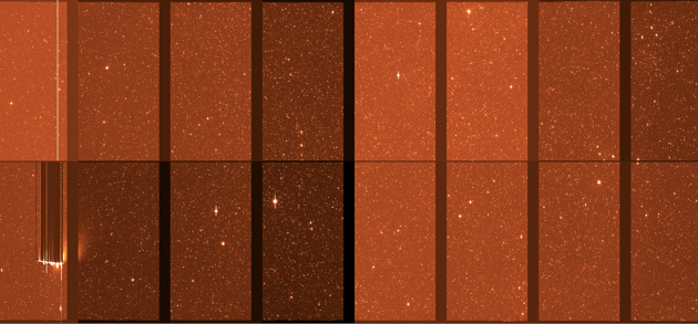
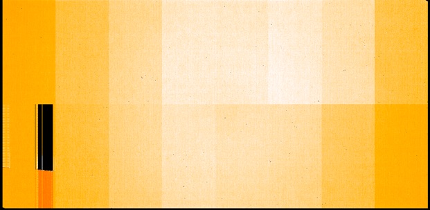
The AST3-1 telescope is equipped with a STA1600 frame transfer CCD with 5280x10560 active pixels, covering 1.5x2.9 degrees on the sky at a scale of 1 arcsec/pixel.  It is readout through 16 amplifiers (each with their own overscan regions) to delivers images like that shown above. I will hereafter refer to each of these sub-images variously as 'channels' or 'chips'.

The frame-transfer time is 0.3s, so each pixel sees the sky during this frame transfer for 0.1ms (in addition to the time it is actually exposed).

The detector has an overall gain of about ~1.8e/adu in its FAST readout mode (the mode used for exoplanet work), though this varies between all the readout channels. The read-noise is ~10e-.

It has a fixed Sloan i-band filter.

DETECTOR TEMPERATURE

Because the AST3-1 peizo-electric coolers run more or less open-loop, the temperature of the the detector will vary over the course of a typical observing run. Thus we can expect dark current, bias levels, detector gain and even linearity to vary with time.

If the bias level behaves the same as other detectors I have used, the actual level of the bias frame (or overscan) will be a function of detector temperature. This can be calibrated from actual data, and may allow the precise measurement of detector temperature for each exposure.

BIAS

Bias levels range from 4000-5000 adu and are different in each channel. No biases are available from Dome A, but its quite clear from the actual data that the detector has the usual complement of hot pixels that will not produce useful data, and which need to be masked out with a bad pixel mask.

AST3-1 has no shutter, so it cannot acquire true BIAS frames while at dome A. On the other hand it can acquire 0s frames that will consist of a reset, followed by a frame transfer and read - in essence a 0.3s exposure. While not a true bias, such observations (if taken when the sky is dark and at multiple telescope positions allowing any bright stars to be medianned out) will tell us the bias levels as a function of time, as well as the stability of hot pixels.

These were not taken as a regular calibration in 2012, but should be part of the daily calibration plan in future campaigns.

DARK CURRENT

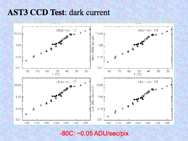
With no shutter, AST3-1 has no way to acquire dark frames. These were acquired in lab testing, and dark count rates measured as a function of detector temperature. The following figure shows some example data

OVERSCAN

Each channel delivers a vertical overscan region to the right of that channel, as well as an overscan at the top and bottom of each channel. Examination of the overscan regions in a few sample images suggests the bias flatness of the channels is very good.

The top overscan of the top channel and the bottom overscan of the bottom channel reveal a 'roll off' in counts that looks more like vignetting of the field edge than a true overscan. It looks like these regions should be ignored for bias estimation purposes.

The 'middle' overscan regions for each channel could be used for horizontal bias pattern examination, and the right regions for vertical estimation.

There is at most a drift of ~1adu in the bias level from the top to the bottom of each channel (i.e. in the vertical direction), and no obvious drift in the horizontal direction.

There is a slight offset between the bias level in the horizontal and vertical overscan regions for each channel. Given there are many less horizontal pixels, I suggest using only the vertical overscan.

Overscan subtraction should be perfectly fine with a single bias level for each channel determined from the side region. At most one could use a linear fit to the vertical overscan, but this would probably be overkill, unless evidence for a vertical pattern is seen.

DEFECTS

As well as a sprinkling of the usual dust artefacts across the detector, there are two large defects that look like a physical crack in the lower-leftmost channel. These essentially kill all columns these cracks lie in for useful astronomy.

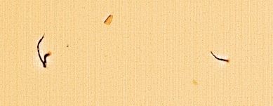
Example artefacts in a flat field resulting from material on the detector surface. These will need to be handled in the data processing system via being flagged as bad for all subsequent processing.

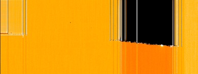
Lower-left channel crack artefact. This kills all data in the entire column affected.

FLAT FIELDS

From looking at combined flat fields prepared by Zhang Hui (Nanjing) its obvious that there are gain offsets between the detectors that will need to be calibrated on a channel-by-channel basis.

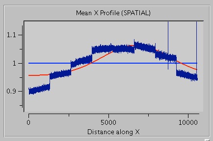
Horizontal cut through the top eight channels. There are differeces of between 3.5 and 10% in gain between adjacent channels.

A quick calculation shows that if these gain differences are taken out, there is an ~4-5% difference in flux detected in the field centre to the field edge. This is an impressively small amount of vignetting at the field edges!

INTER-CHANNEL CROSSTALK

There is significant cross-talk between the channels - this manifests as saturated regions producing regions of flux decrement in the "electronically equivalent locations" in all the other channels.

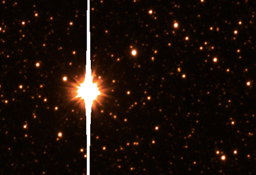
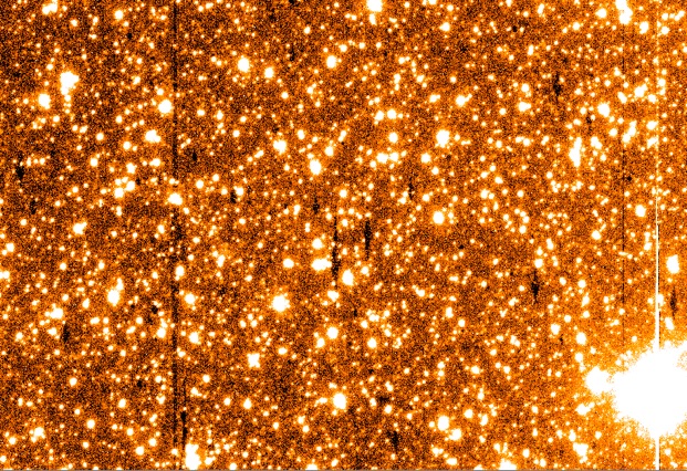
Bright Star in one channel

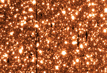
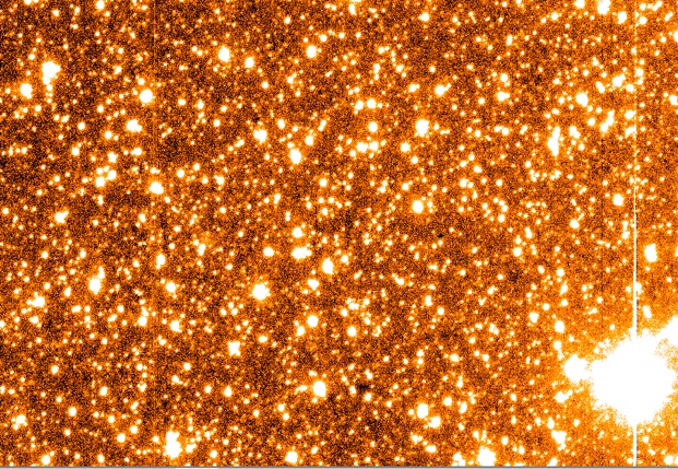
Ghost from it in another channel. The "flux decrement" in the darker regions are about 50adu below the sky level. Note that because each saturated star ghosts into every channel, the wide field of view means that every channel sees a lot of ghosts. Some of these are quite small and could mimic star-sized objects.

These will need to be corrected.

Just what "electronically equivalent" means for the positions of these ghosts is shown below.

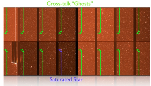
Note that this cross-talk is clearly driven by the operation of the electronics - ghosts of the saturated features produced by the crack in the lower-left channel are also seen in every channel - so the ghosts are not just driven by the detection of photons, but by the electronics that records charge from the detector.

This also means you need to correct the ghosts first before you mask out bad regions!

Correcting this cross-talk will be critical for image processing steps that involve difference imaging, as the negative artefacts the cross-talk produces can be quite small, and so mimic a positive detection in a difference image.

Fortunately, correcting for these ghosts seems to be straight forward using following algorith.

1. 1. Mask each image to determine which pixels are saturated (i.e. have value 65535 or higher) - set these pixels to 65535 and all other pixels to 0.
   

2. 2. Slice the image into its constituent channels (flipping the top channels vertically) and add  them all together to make a single image that reflects the positions of all the saturated stars in the entire images.
   

3. 3.Redistribute this image into all 16 channels (flipping the top channels) to produce a copy of the original image showing the locations of all ghosts.
   

4. 4.Multiply this image by a 'fudge factor' (1.e-3 has been tried and works reasonably well), and add it to the original raw image to produce a cross-talk corrected image.
   

This has been implemented (as a Perl Data Language script) and tested for two raw images made available on May 30, and works remarkably well. The following two images show the same ghost region as above, and a corrected version of it.

Further testing needs to be done with data from many nights to determine whether the 'fudge factor' changes from night to night. My experience with this effect in other multi-amplifier systems suggests it should be quite stable.

In any case it is *strongly* recommended that a cross-talk map be carried through the data processing with each image, so that any unusual objects can be cross-checked against it when they are selected from the later imaging database.

LINEARITY

Exoplanet science (or at least transit observations) rely critically on being able to obtain high precision photometry for the brightest stars in each observing field. This means the detectors must be able to be linearised over their full well depth, so that photometry is independent of seeing.

Limited linearity data is available at present, based on test observations obtained in AST3-1's lab testing before shipping to Dome A. The following figure summarises these results for two channels.

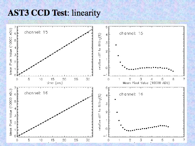
Two points are immediately obvious

1. 1.The detectors show the usual behaviour of returning less counts than expected at high count rates.
   

2. 2.The difference between the countrates returned at low counts (<10000 adu) and high countrates (>30000 adu) are very large - up to 5%.
   

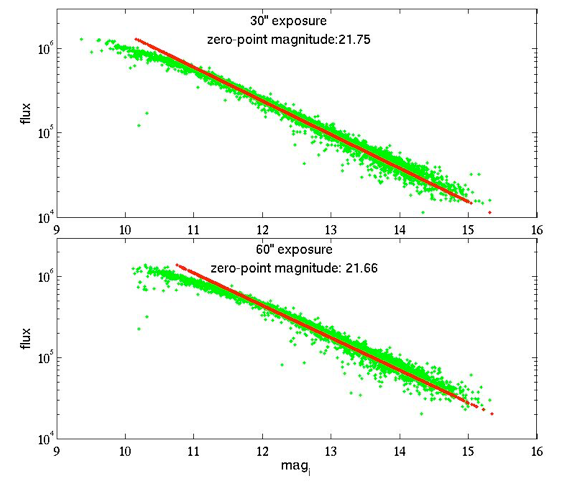
These trends need to be understood in details, and corrections for them included in any pipeline, otherwise the AST3 will be essentially useless of exoplanet transit work. As an example of this, here is a calibration curve between un-linearity-corrected photometry and APASS i' photometry. The 'droop' at the bright end is a pretty clear sign that non-linearity is setting in and severely compromising the photometry.